2D Object Detection - Experiments

Welcome to my blog post where I’ll be sharing my insights into 2D object detection. This post will cover what 2D object detection is, the latest advancements in the field, how we measure the performance of detection algorithms, a deep dive into YOLO algorithms, and my experience building YOLOv1 from scratch. We’ll also explore important datasets like nuImages, and I’ll share some handy tools I’ve picked up along the way, including Weights & Biases, Docker, and our server to train neural networks called “Deep LAR”. I’ll also describe the next steps of my PhD journey and discuss what we can expect from it. Let’s dive in and explore the world of 2D object detection.

Definition of 2D Object Detection

2D object detection is a fundamental task in computer vision, focusing on identifying and pinpointing objects within images or video frames. Its applications span various fields such as surveillance, autonomous driving, and robotics. This task broadly categorizes algorithms into two types: single-shot detectors and two-shot detectors, depending on how they process input images.

Single-shot object detection involves analyzing the entire image in a single pass to determine the presence and location of objects. This method, is computationally efficient and suitable for real-time applications. However, it tends to be less accurate, especially for detecting small objects. The most famous single-shot object detection algorithm is YOLO (You Only Look Once) [1].

On the other hand, two-shot object detection operates in two stages. Initially, it generates a set of potential object locations or proposals. In the subsequent pass, these proposals are refined to produce final predictions. While offering higher accuracy, this approach is more computationally intensive. The most famous two-shot object detection algorithm is the RCNN [2].

The division of the 2D object detection task is exemplified in figure 1, with the most known algorithms. In summary, the choice between single-shot and two-shot object detection hinges on the specific requirements of the application: real-time processing versus accuracy.

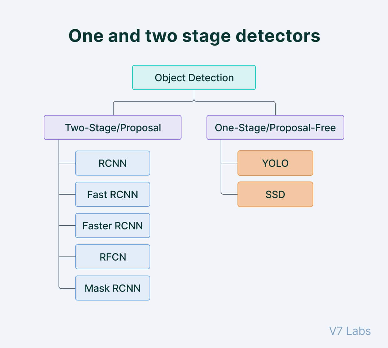Figure 1: Types of 2D object detection [3]

Evaluation metrics for 2D object detection

In assessing the performance of 2D object detection models, two primary evaluation metrics stand out: Intersection over Union (IoU) and Average Precision (AP).

Intersection over Union (IoU)

IoU serves as a fundamental metric for measuring localization accuracy in object detection. It quantifies the overlap between predicted and ground truth bounding boxes, exemplified in Figure 2. By calculating the ratio of the area of intersection to the area of union between the two bounding boxes, IoU provides insight into how closely the predicted bounding box aligns with the actual object location.

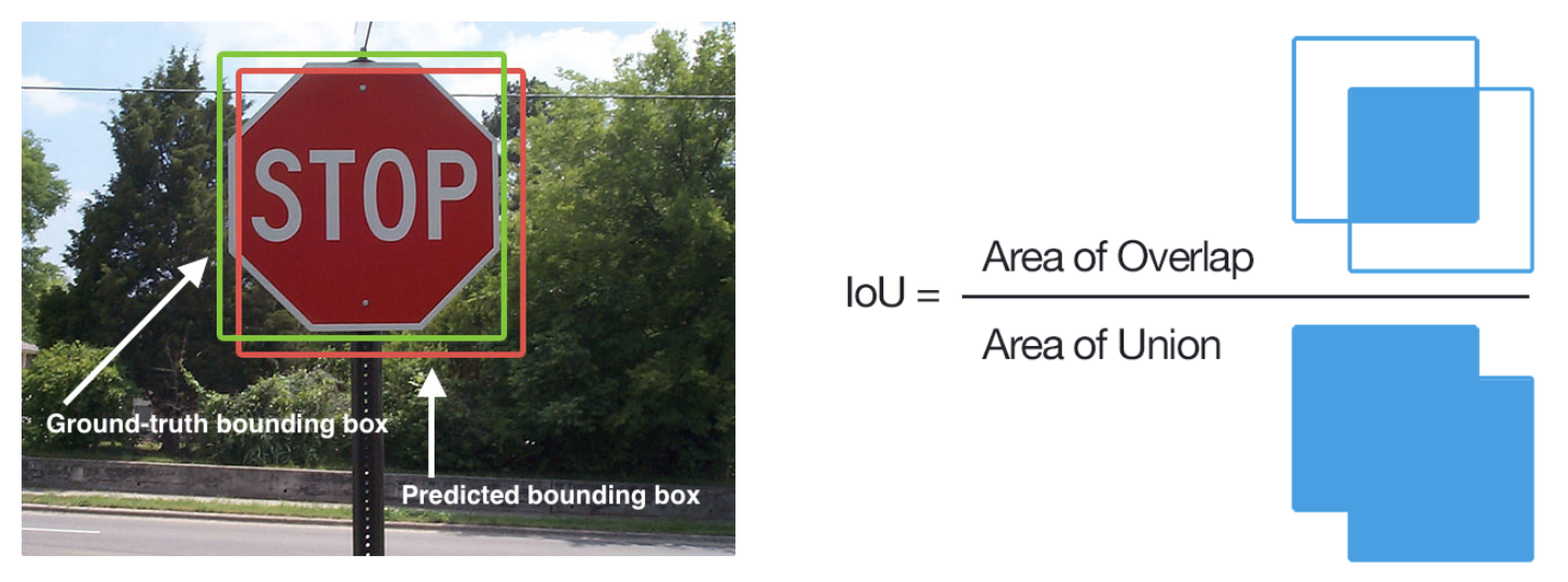Figure 2: Intersection over Union (IoU) Illustration [4]

Average Precision (AP)

Average Precision is derived from the precision-recall curve and offers a comprehensive evaluation of detection performance. Precision represents the ratio of true positives to the total predictions made by the model, while recall accounts for the ratio of true positives with respect to the total ground truth objects. The difference between precision and recall is exemplified in Figure 3. By varying the classification threshold, we generate a precision-recall curve, and the area under this curve yields the Average Precision per class. The mean Average Precision (mAP) is the average of AP values across all classes.

Figure 3: Precision and Recall Illustration [3]

In object detection, precision and recall are not employed for class predictions but for bounding box predictions. An IoU threshold is utilized to distinguish positive predictions from negative ones, enabling accurate measurement of decision performance based on bounding box localization.

YOLO algorithms

YOLOv1

YOLO (You Only Look Once) revolutionized object detection by processing images in a single pass. Its architecture involves pre-training the first 20 convolutional layers using ImageNet, followed by converting the model for detection tasks. YOLO divides images into an S × S grid, with each grid cell responsible for predicting bounding boxes and confidence scores for objects within it. This model utilizes non-maximum suppression (NMS) to refine predictions and remove redundant bounding boxes.

Figure 4: YOLOv1 architecture [1]

YOLOv2

YOLOv2 introduced anchor boxes for handling a variety of object sizes and aspect ratios. It also incorporated batch normalization and a multi-scale training strategy to enhance model stability and detection performance.

YOLOv3

YOLOv3 adopted the Darknet-53 architecture and introduced anchor boxes with diverse scales and aspect ratios. Additionally, it incorporated feature pyramid networks (FPN) to detect objects across multiple scales, improving performance on smaller objects.

YOLOv4

YOLOv4 featured the Cross Stage Partial Network (CSPNet) architecture and utilized k-means clustering for anchor box generation. It introduced the GHM loss function which is designed to improve the model’s performance on imbalanced datasets.

YOLOv5

YOLOv5 employed the EfficientNet architecture and dynamic anchor boxes for higher accuracy and generalization. It introduced spatial pyramid pooling (SPP) and CIoU loss to enhance detection performance, especially on small objects.

YOLOv6

YOLOv6 utilized the EfficientNet-L2 architecture and dense anchor boxes for efficient object detection.

YOLOv7

YOLOv7 incorporated focal loss to handle small object detection effectively and operated at a higher image resolution for improved accuracy.

YOLOv8

YOLOv8 introduced the CSPDarknet53 backbone and PANet neck network for enhanced feature representation and object identification. Its architectural changes and refined loss algorithms contributed to improved precision and stability in object detection tasks.

These iterations of the YOLO algorithm demonstrate a continual evolution towards better accuracy, efficiency, and versatility in object detection.

Implementation of YOLOv1 from scratch

For a comprehensive understanding of YOLO and its metrics, I embarked on a tutorial to implement YOLOv1 from scratch using PyTorch. This hands-on approach allowed me to delve deep into the practical implementation of YOLO and its associated evaluation metrics.

Throughout the implementation process, I gained valuable insights into structuring deep learning projects, including the creation of auxiliary functions and classes for dataset processing, model construction, configuration files, and custom loss functions.

Following the tutorial, I refined the training script to suit my preferences, enhancing its completeness and incorporating an inference script for evaluating trained models. I also improved result visualization and incorporated the use of Weights & Biases for metric tracking and result visualization.

Key highlights of the implementation include:

• Creation of custom classes for dataset processing tailored to PascalVOC and NuImages datasets.
• Implementation of YOLOv1 model architecture and custom loss function.
• Optimizations in the training code, including the addition of time elapsed tracking, best model saving, and results visualization.
• Integration with Weights & Biases for comprehensive metric tracking.
• Adoption of best practices in project organization, with dedicated directories for datasets, models, repositories, and results.
• Implementation of YOLOv1 with a pre-trained ResNet50 backbone to facilitate training.
• Adaptation of the NuImages dataset into a custom PyTorch dataset compatible with YOLOv1.

These implementations not only provided a thorough understanding of YOLOv1 but also equipped me with reusable code and best practices that will streamline future tasks and implementations. I also got I overview understanding about hyperparameters search and tuning. Now, I will present the results obtained from applying the YOLOv1 algorithm on both the PascalVOC and NuImages datasets.

In the PascalVOC dataset, after training for 135 epochs, I achieved an mAP of 16.07%. Although this result falls short of the 57.9% reported by the authors in the paper, it’s important to note that I didn’t dedicate extensive time to hyperparameter tuning. Additionally, the authors employed data augmentation techniques to enhance their results, which I did not explore thoroughly. For a visual representation of the training progress, Figures 5 and 6 illustrate the training/validation loss and validation mAP across epochs, respectively. In this link there are the results to compare side by side the predicted bounding boxes and the ground truth bounding boxes.

Figure 5: train/val loss over epochs in PascalVOC dataset

Figure 6: val mAP over epochs in PascalVOC dataset

The outcomes obtained from the NuImages dataset were disappointing, albeit not entirely unexpected. This dataset poses significantly greater challenges compared to PascalVOC, featuring numerous small objects that are inherently harder to detect—a limitation of the YOLOv1 algorithm. Despite training for 135 epochs, we only attained a meager mAP of 0.12%. It’s worth noting that, similar to the PascalVOC experiment, I didn’t allocate ample time for hyperparameter tuning. However, it’s evident that YOLOv1 isn’t ideally suited for this dataset due to its inherent limitations in detecting small objects effectively. For a visual representation of the training progress, Figures 7 and 8 illustrate the training/validation loss and validation mAP across epochs, respectively. In this link there are the results to compare side by side the predicted bounding boxes and the ground truth bounding boxes. The source code to all these experiments can be seen on GitHub.

Figure 7: train/val loss over epochs in nuImages dataset

Figure 8: val mAP over epochs in nuImages dataset

nuImages - Autonomous Driving Dataset

The nuImages dataset stands as a pivotal resource in the realm of autonomous driving research, renowned for its extensive use in end-to-end perception algorithms. Selected as a benchmark dataset for my PhD endeavors, nuImages offers a comprehensive collection of images annotated with 2D bounding boxes and masks, facilitating nuanced analysis and algorithm evaluation.

Key features of the nuImages dataset include:

• Dataset Composition: Comprising 93,000 images, nuImages is subdivided into 67,000 training images, 16,000 validation images, and 10,000 test images, ensuring a robust and diverse dataset for algorithm development and evaluation.
• Data Collection: The dataset originates from nearly 500 logs of driving data, far surpassing its predecessor, nuScenes, which contained 83 logs. This extensive collection allows for a broader representation of real-world driving scenarios.
• Annotation Strategy: Employing active learning techniques, approximately 75% of the images are intentionally selected to present challenges based on the uncertainty of image-based object detectors. Emphasis is placed on rare classes like bicycles to enhance model robustness. The remaining 25% of images are uniformly sampled to ensure dataset representativeness and mitigate biases.
• Curation and Quality Control: Rigorous curation of the dataset is conducted to ensure diversity in terms of class distribution, spatiotemporal distribution, and weather and lighting conditions. Images exhibiting camera artifacts, low illumination, or pedestrian faces are carefully reviewed and discarded as necessary.
• Temporal Dynamics: Each annotated image in nuImages is accompanied by six past and six future camera images, captured at a frequency of 2 Hz. This temporal context enables researchers to study dynamic scene changes and enhance understanding of real-time driving scenarios.

By providing a rich and meticulously curated dataset, nuImages serves as an indispensable resource for advancing research in autonomous driving, facilitating the development and evaluation of state-of-the-art perception algorithms. Figure 9 illustrates the database schema of nuImages and Figure 10 shows an example of the annotations provided by nuImages.

Figure 9: nuImages schema

Figure 10: nuImages annotation example

Auxiliary tools learned during this task

Weights & Biases (wandb)

Weights & Biases (W&B) serves as a vital tool for training and fine-tuning perception algorithms in 2D object detection. It offers a range of functionalities tailored to streamline the development process. W&B provides a user-friendly AI developer platform equipped with tools designed to enhance model training, fine-tuning, and experimentation. The key features of W&B are:

• Experiment Tracking: W&B enables meticulous tracking of experiment progress, allowing real-time monitoring of metrics such as loss, accuracy, and validation scores during training.
• Hyperparameter Optimization: With W&B, users can systematically search for the optimal set of hyperparameters, facilitating the enhancement of model performance.
• Model Visualization: The platform offers robust visualization capabilities, enabling users to plot results, including bounding boxes, for comprehensive analysis and interpretation.

Docker

Docker is a platform that enables containerization—a technique that encapsulates software and dependencies into isolated units called containers. These containers can run on any machine without modification, providing consistency across different computing environments. Docker streamlines machine learning (ML) deployment by encapsulating software and dependencies into isolated containers. It resolves compatibility issues and ensures consistent performance across diverse environments. Docker facilitates interoperability, scalability, and portability, allowing ML models to seamlessly integrate into complex architectures and deploy across distributed systems. It simplifies version control, enabling efficient management of container images and facilitating collaboration. With Docker, ML applications exhibit fault tolerance and continuous deployment, enhancing operational reliability and efficiency.

Deep LAR

DeepLAR is a purpose-built computer designed to serve as a deep learning server for researchers at the Laboratory for Automation and Robotics (LAR), housed within the Department of Mechanical Engineering at the University of Aveiro. This powerful computing system boasts an array of GPU resources, enabling the development of machine learning algorithms. The specifications of DeepLAR are as follows:

• 4 x NVIDIA RTX2080TI GPUs
• AMD Threadripper 2850 Extreme Processor
• 128GB DDR4 RAM
• 512GB SSD + 4TB HDD Storage Configuration

What’s next?

I believe it’s crucial to maintain continuity in our exploration of image processing, transitioning from 2D object detection to 2D object tracking in images. This progression will pave the way for further advancements, including venturing into the realm of 3D object detection and subsequently 3D object tracking using LiDAR technology and point clouds.

References

[1] J. Redmon, S. Divvala, R. Girshick and A. Farhadi, “You Only Look Once: Unified, Real-Time Object Detection,” 2016 IEEE Conference on Computer Vision and Pattern Recognition (CVPR), Las Vegas, NV, USA, 2016, pp. 779-788, doi: 10.1109/CVPR.2016.91.

[2] R. Girshick, J. Donahue, T. Darrell and J. Malik, “Rich Feature Hierarchies for Accurate Object Detection and Semantic Segmentation,” 2014 IEEE Conference on Computer Vision and Pattern Recognition, Columbus, OH, USA, 2014, pp. 580-587, doi: 10.1109/CVPR.2014.81.

[3] YOLO: Algorithm for Object Detection Explained

[4] Mean Average Precision (mAP) Explained: Everything You Need to Know

[5] nuImages dataset