Motion Prediction - Experiments

In this post, I will delve into the critical topic of motion prediction in autonomous vehicles. Motion prediction plays a pivotal role in enabling self-driving cars to anticipate the movements of surrounding road users, thereby enhancing safety and efficiency. This post will cover several key aspects of motion prediction, including its definition, the challenges involved, the datasets used for training and benchmarking, the evaluation metrics used to assess the algorithms, the state-of-the-art approaches, the experiments conducted in this perception task and finally what are the next steps in my PhD progress. Let’s dive in and explore how motion prediction is shaping the future of autonomous driving.

Definition of motion prediction

Motion prediction in the context of autonomous driving refers to the process of forecasting the future positions and trajectories of surrounding vehicles and other road users. This predictive capability is crucial for enabling autonomous vehicles to navigate safely and efficiently by anticipating potential hazards and planning appropriate maneuvers. The primary goal of motion prediction is to enhance the vehicle’s understanding of the dynamic environment, thereby reducing uncertainty in decision-making and improving overall safety and comfort.

Expressions related to “motion prediction” include “behavior prediction,” “maneuver prediction,” and “trajectory prediction.” Behavior prediction is a more general term that encompasses both maneuver prediction and trajectory prediction. Trajectory prediction specifically outputs the coordinates of the target agent’s future path over a certain time period. In contrast, maneuver prediction attempts to infer possible future maneuvers or intentions of the target agent. Both trajectory and maneuver predictions focus on individual-level forecasts. In this context, vehicle motion prediction refers to estimating the motion state sets of target vehicles within a fixed future horizon based on available scene information acquired by the ego vehicle.

Deep learning-based methods have become the dominant approach for vehicle motion prediction, thanks to their ability to process complex scene information and achieve long-term predictions. Initially, the model inputs the available scene information during the observation stage. This information is then processed by the scene context encoder, which encodes the inputs and extracts context features related to the future motion of target vehicles (TVs). The motion predictor subsequently decodes the fully extracted context features to generate the prediction outputs.

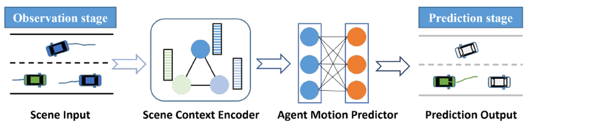Figure 1: An illustration of the DL-based motion prediction paradigm. The green vehicle is the target vehicle. The input here includes the historical trajectories of vehicles and the road structure, and the output is the future trajectory. [1]

Challenges of motion prediction

Motion prediction for autonomous driving involves several significant challenges, each arising from the complexity and dynamic nature of real-world driving scenarios. Here are the main challenges:

1. Inter-dependency and Complex Interactions: Vehicles on the road constantly interact with one another, creating inter-dependencies and complex interactions within the scene. For example, when a target vehicle (TV) plans to change lanes, it must consider the driving states of surrounding vehicles. Similarly, the lane-change action taken by the TV will affect the surrounding vehicles. Therefore, an effective prediction model needs to account for the states of all involved vehicles and their interactions within the scene.

2. Multimodal Nature of Vehicle Motion: Vehicle motion is inherently multimodal due to the variability in drivers’ intentions and driving styles. This introduces a high degree of uncertainty in predicting future motions. For instance, at a junction, a vehicle might go straight or turn right despite having similar historical input data. Additionally, different driving styles can result in varying speeds for the same maneuver. Current motion prediction methods often use multimodal trajectories to represent this diversity. These models must effectively explore and cover all possible trajectories that a vehicle might take.

3. Constraints from Static Map Elements: Future motion states of vehicles are often constrained by static elements such as lane structures and traffic rules. For example, vehicles in right-turn lanes must perform right turns. Models should integrate map information to extract full context features relevant to the future motion of the vehicles, ensuring adherence to traffic rules and lane structures.

4. Predicting Multiple Vehicles: In dense traffic scenarios, it is necessary to predict the motion states of several or all vehicles around the ego vehicle (EV). This requires models to jointly predict multiple target agents, with the number of target vehicles (TVs) varying according to the current traffic conditions. The joint prediction must also ensure coordination between vehicles to avoid overlaps in their future trajectories.

5. Complexity of Encoding Input Information: Deep learning-based methods can handle various types of input information, but as the type and number of inputs increase, the complexity of encoding these inputs also rises. This can lead to confusion in learning different types of information. The prediction model needs to efficiently and adequately represent the input scene information to better encode and extract features. Extracting the full context feature from pre-processed input information remains an open challenge in the field.

6. Practical Deployment Challenges: Deploying prediction models in real-world scenarios poses several practical challenges. Firstly, many models assume complete observation of relevant vehicles (RVs), but in reality, vehicle tracks may be missed due to occlusion. Accurate prediction based on incomplete input is still a problem. Secondly, many prediction methods treat prediction as an independent module, lacking integration with other modules of autonomous driving systems. Lastly, there is the issue of timeliness, especially for complex deep neural networks that consume significant computational resources, potentially impacting real-time performance.

These challenges highlight the complexity of motion prediction in autonomous driving and the need for advanced models that can handle the diverse and dynamic nature of real-world driving scenarios.

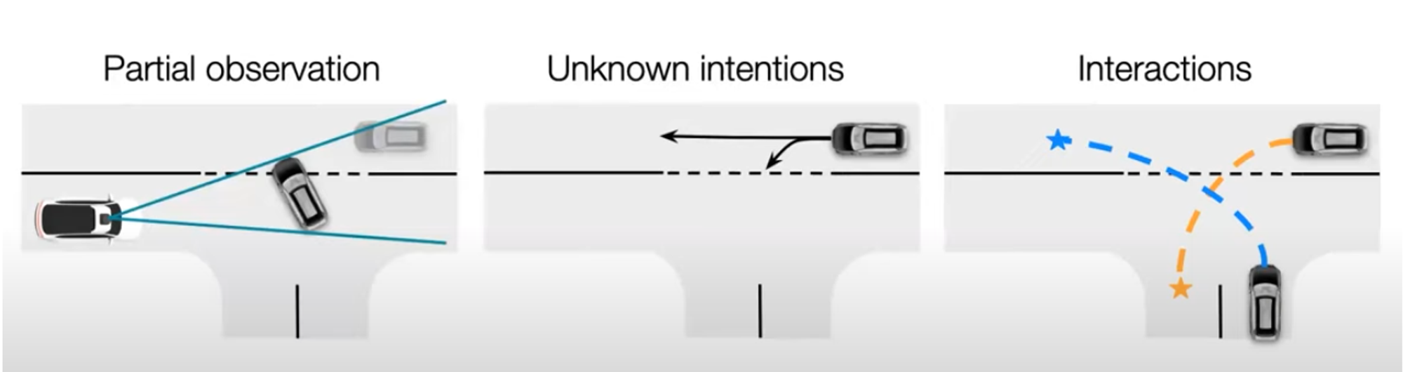Figure 2: Main challenges of motion prediction. [2]

State of the art

The state of the art in vehicle motion prediction focuses on overcoming several critical challenges. This section delves into the key areas: scene input representation, context refinement, and prediction rationality improvement.

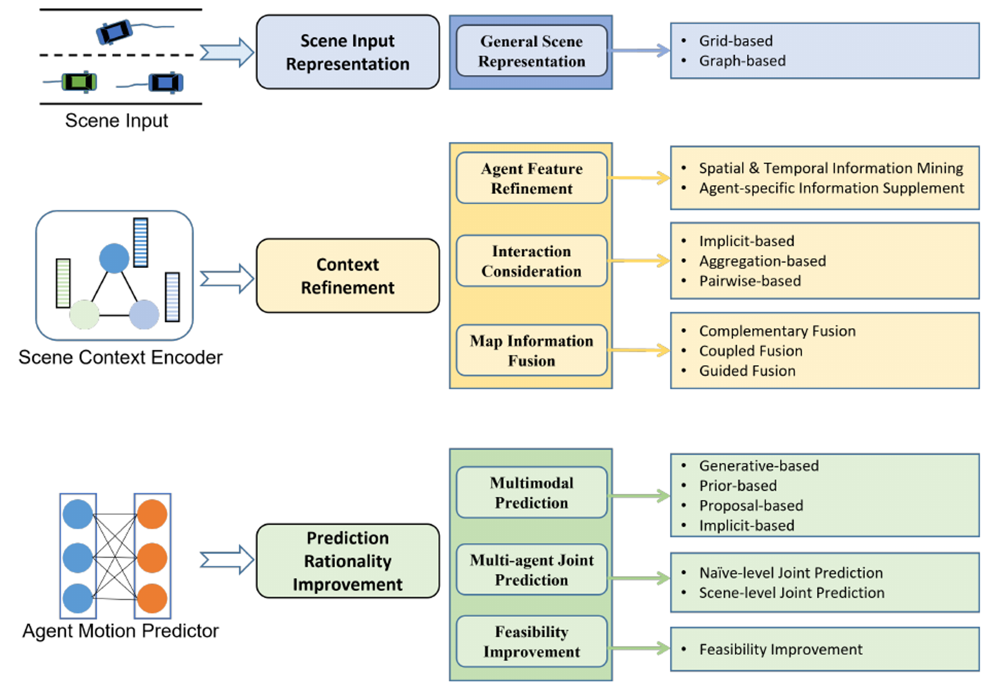Figure 3: The classification for vehicle motion prediction methods. [1]

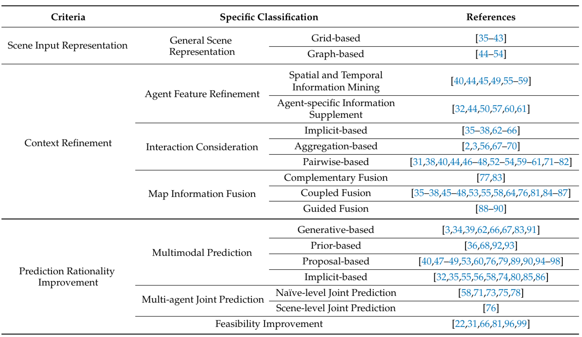Figure 4: Overall distribution of covered literature. [1]

Scene Input Representation

Scene input refers to the surrounding environment information acquired within the perceptible range by the ego vehicle (EV), including the historical motion states of traffic participants and map information. The prediction model needs to encode features based on a reasonable scene representation. As the input becomes richer and more diverse, some works construct a general representation of all scene elements to reduce model complexity and improve the efficiency of feature extraction. Recent works for general scene representation can be classified into grid-based and graph-based approaches.

---

Grid-Based

The grid-based approach divides the region of interest into regular and uniformly sized grid cells, each storing information about the area, such as encoded historical motion features of vehicles within the cell. This representation emphasizes the spatial proximity between scene elements, preserving scene information as richly as possible. By organizing data in this way, the prediction model can capture spatial relationships effectively and easily integrate other region-based input information.

Grid-based representations are often encoded using convolutional neural networks (CNNs), which have mature network frameworks that facilitate implementation. However, this method typically generates actor-specific representations, which are not easily extended to multi-agent joint prediction. Additionally, the convolutional kernels used in these models are generally limited in size to manage complexity, potentially leading to the omission of long-range information.

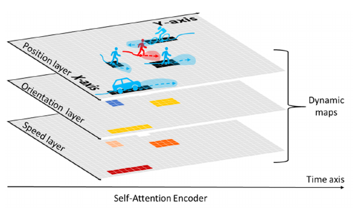Figure 5: An example of grid-based representation. The authors design a 3-channel grid map to encode the location, orientation, and speed of traffic participants in the space around the target agent. [1]

Graph-Based

Given the variability and non-regularity of road structures, and the diverse, implicit, and complex interrelationships between elements within a scene, some works use graphs to represent scenes. Graph-based representation constructs a scene graph that fully reflects the interrelationships of scene elements. The scene graph is composed of nodes and edges, where nodes represent specific objects and edges describe the relationships between nodes.

Graph-based representation is sparser than grid-based representation and highlights the flow of spatial-temporal information. Models using this approach can consider a more extended range of scene information by transmitting and updating node features multiple times. However, this approach requires predefined node connection rules, such as undirected full connection rules for agent nodes and spatial connectivity rules for lane nodes. Defining suitable connection rules can be challenging when scene elements are diverse and have complex relationships.

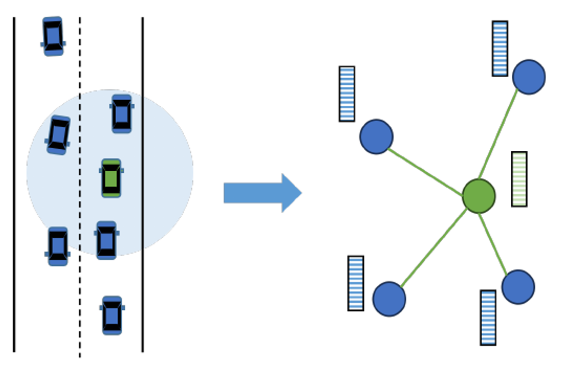Figure 6: An example of graph-based representation. The green vehicle is the target to be predicted, while blue vehicles belong to surrounding vehicles. A scene graph centered on the target vehicle is constructed to capture the interactions. Nodes represent agents in the scene, and an edge exists if the distance between a surrounding vehicle and the target vehicle is below a threshold. [1]

---

Both grid-based and graph-based approaches offer unique advantages and limitations. Grid-based methods benefit from well-established CNN frameworks and effective spatial relationship modeling but may struggle with multi-agent predictions and long-range interactions. Graph-based methods excel at capturing complex, non-Euclidean relationships but require careful definition of connection rules and may be computationally intensive.

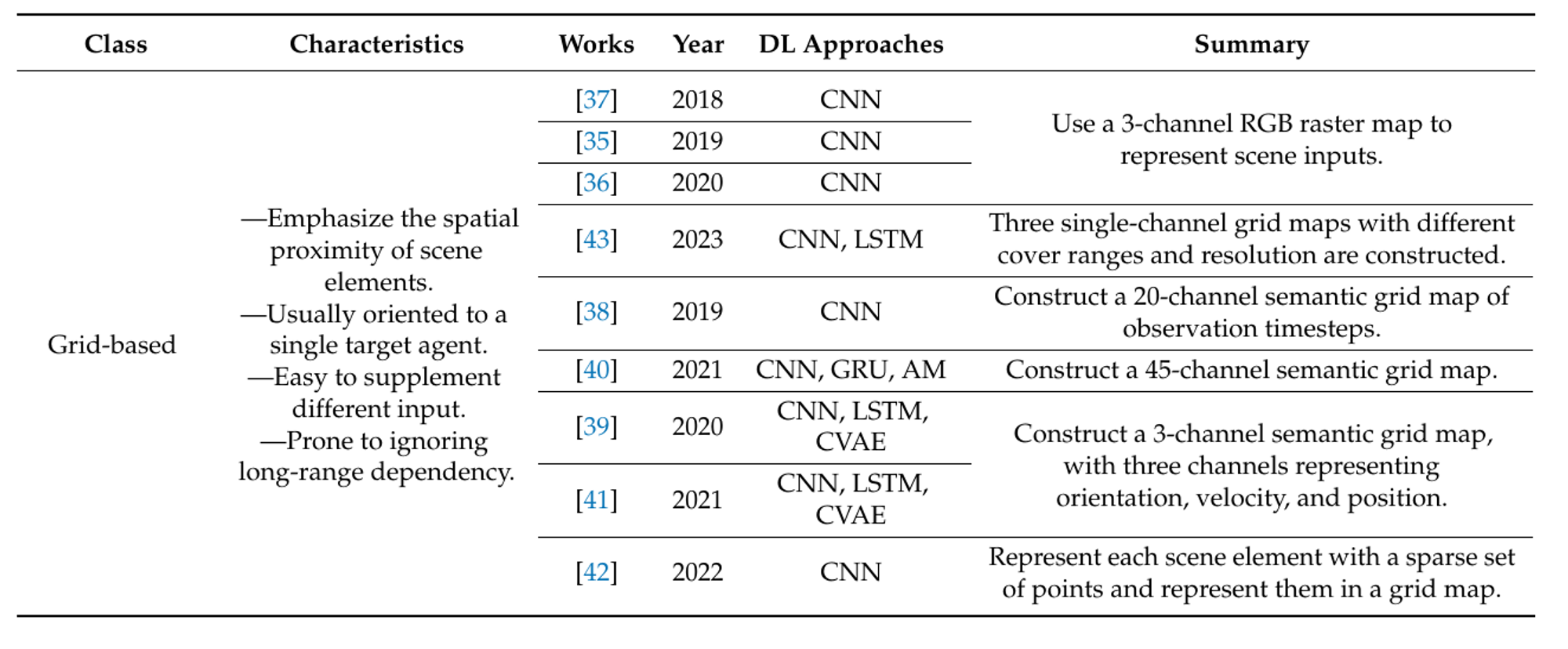
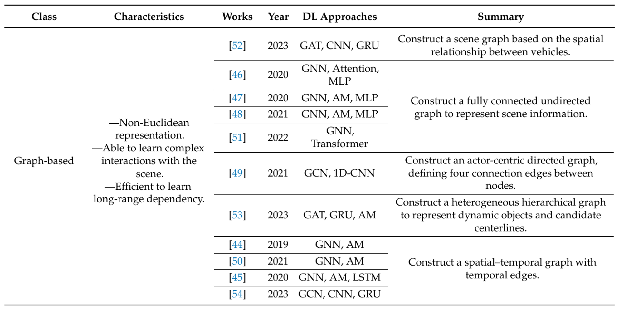Figure 7: Summary of General Scene Representation methods of recent works. [1]

Context refinement

The scene context refers to the abstract summary of scene information, particularly relevant to motion prediction. Extracting the scene context involves learning both historical static and dynamic information about the scene. This section summarizes context refinement methods from three aspects: Agent Feature Refinement, Interaction Consideration, and Map Information Fusion.

Agent Feature Refinement

Deep learning-based prediction models need to encode individual features of dynamic agents to fully extract the scene context. Adequate extraction of agent features facilitates the acquisition of the scene context. The methods for refining the extraction of individual agent features are divided into two classes: Spatial and Temporal Information Mining and Agent-Specific Information Supplement.

Spatial and Temporal Information Mining: Vehicles are carriers of spatial-temporal states, necessitating careful consideration of agent information across both dimensions. Neglecting either spatial or temporal information can be detrimental to the extraction of the context feature. Emphasizing the spatial-temporal characteristics of the vehicle allows for the exploration of full spatial-temporal features.

Agent-Specific Information Supplement: Refinement of agent features can also involve encoding agent-specific information, such as supplementing input with category attributes of different traffic participants. This optimization of individual agent feature extraction ensures specific agent information is adequately considered.

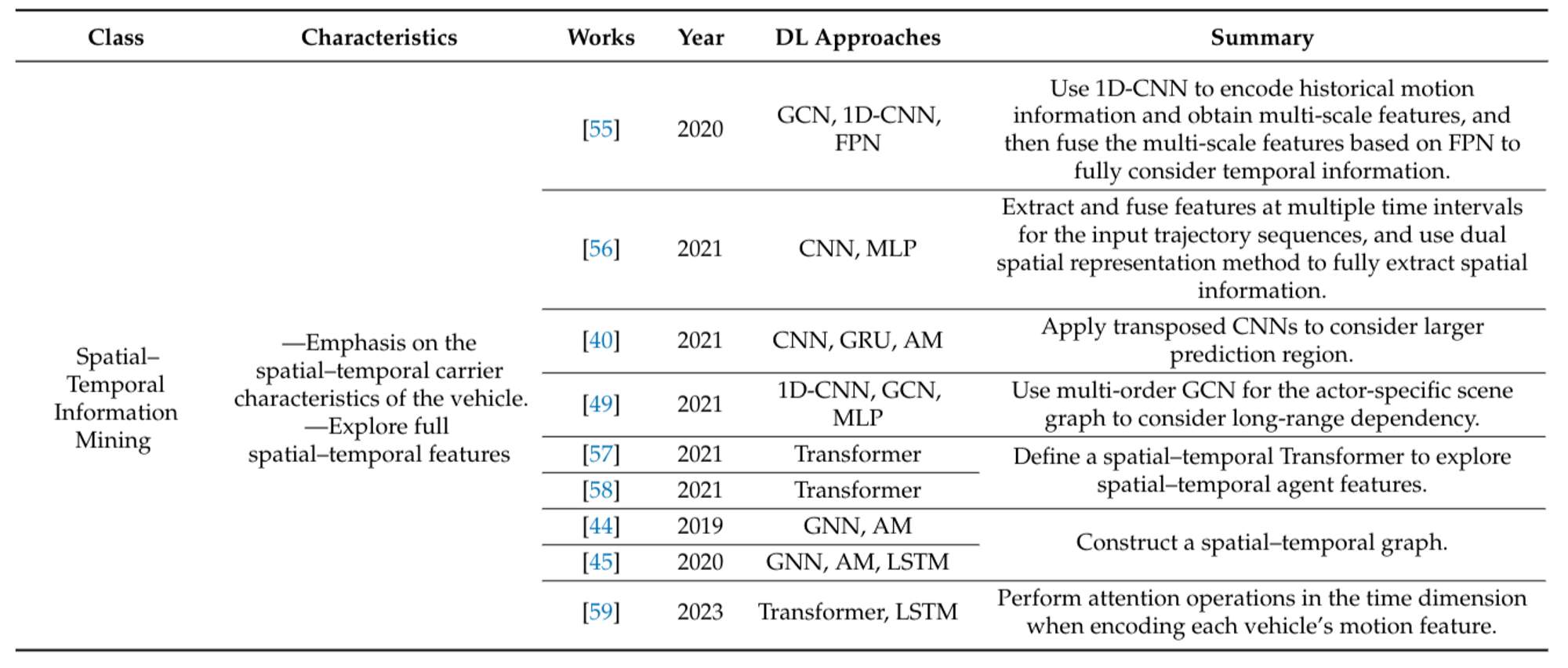
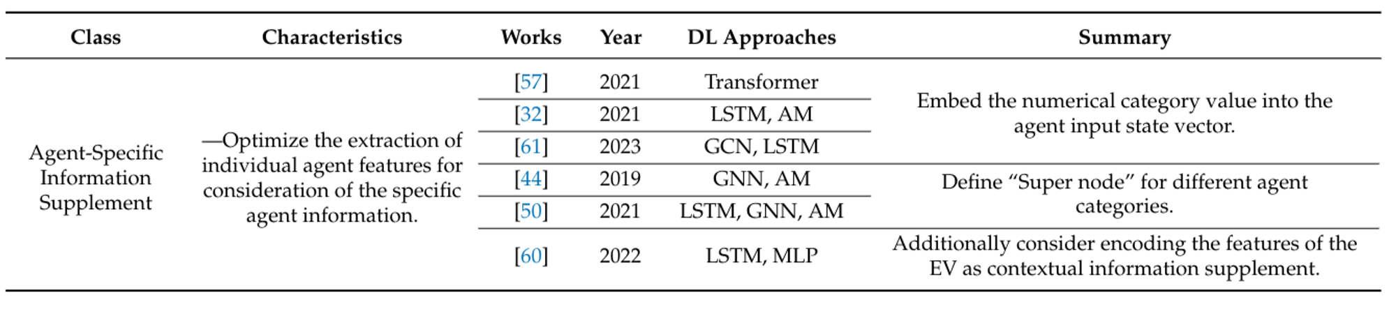Figure 8: Summary of agent feature refinement methods of recent works. [1]

Interaction Consideration

Interactions between agents, or inter-dependencies, refer to the mutual influences among agents in the same space-time. Learning interaction information helps models refine the context feature. Current methods of interaction consideration are divided into three categories: implicit-based, aggregation-based, and pairwise-based.

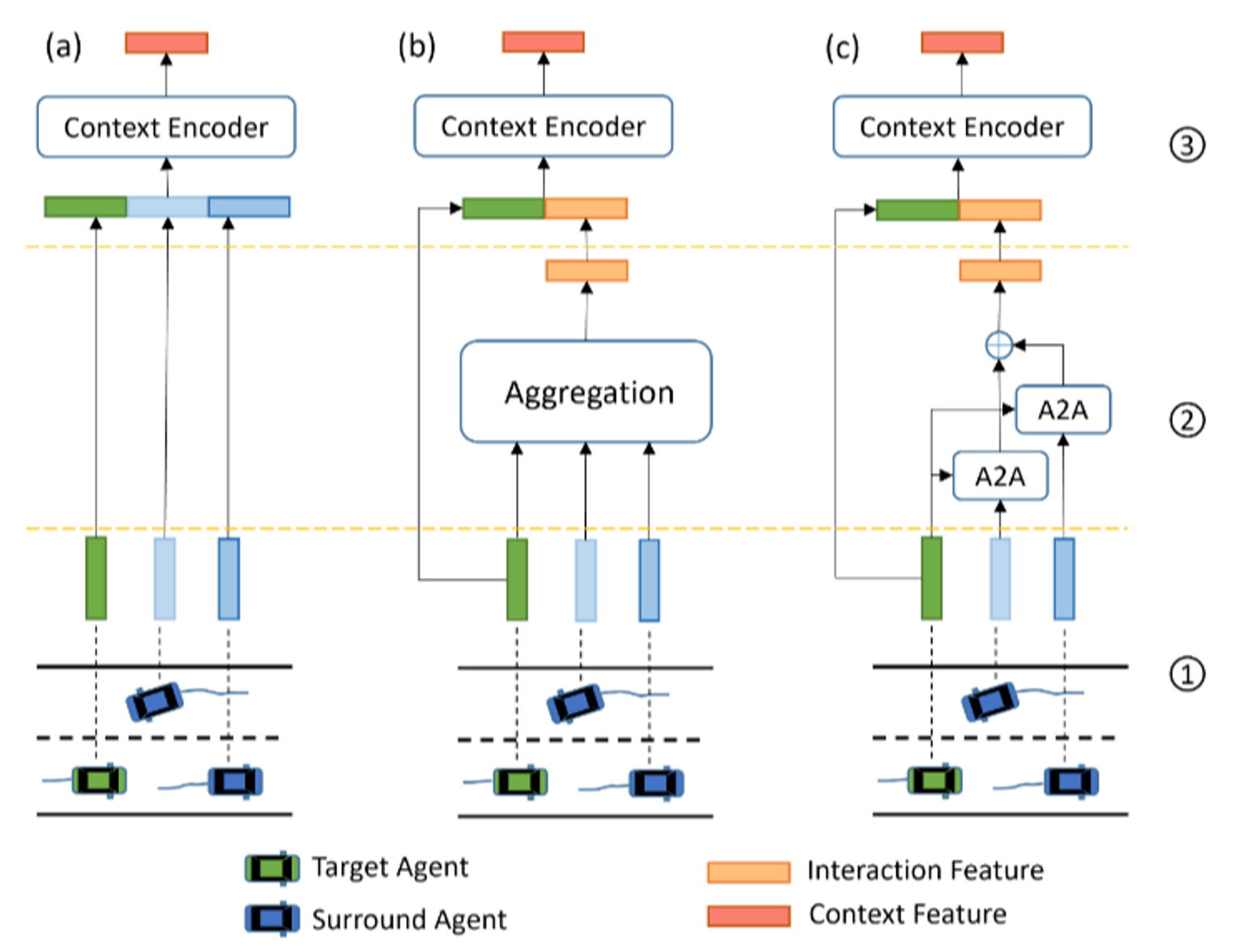Figure 9: An illustration of interaction consideration methods: (a–c) denote implicit-based, aggregation-based, and pairwise-based methods, respectively. Numbers 1, 2, and 3 denote the agent feature encoding stage, interaction feature encoding stage, and context feature encoding stage, respectively. The implicit method has no explicit interaction feature encoding phase. In aggregation-based methods, the features of vehicles around the target vehicle are aggregated in a uniform manner such as averaging pooling to obtain the interaction feature and then concatenated with the target vehicle feature to obtain the context feature. The pairwise-based method designs agent-to-agent (A2A) modules to model the different inter-dependencies between each surrounding agent and the target agent. The A2A module is usually based on the attention mechanism. [1]

Implicit-Based: Implicit-based interaction consideration does not explicitly compute the interaction feature. Instead, the model considers the states of other traffic participants around the target agent to extract the context feature, assuming the extracted feature already contains interaction information. This approach is easy to implement but has drawbacks, such as insufficient interaction learning and an inability to distinguish between different influences from other vehicles.

Aggregation-Based: The aggregation-based approach explicitly encodes the interaction feature through a two-stage process: first encoding the motion states of each vehicle of interest, then aggregating these features to represent the interaction influence on the target vehicle. While this approach explicitly considers spatial correlation, it often limits interaction information to a fixed spatial range and fails to distinguish between the influences of different agents.

Pairwise-Based: The pairwise-based approach highlights specific inter-dependencies between two agents. It integrates the influence of surrounding vehicles on the target vehicle efficiently, often using attention mechanisms or graph neural networks. The former functions similarly to a weighted sum of surrounding agent information, while the latter focuses on aggregating, passing, and updating features of surrounding agents.

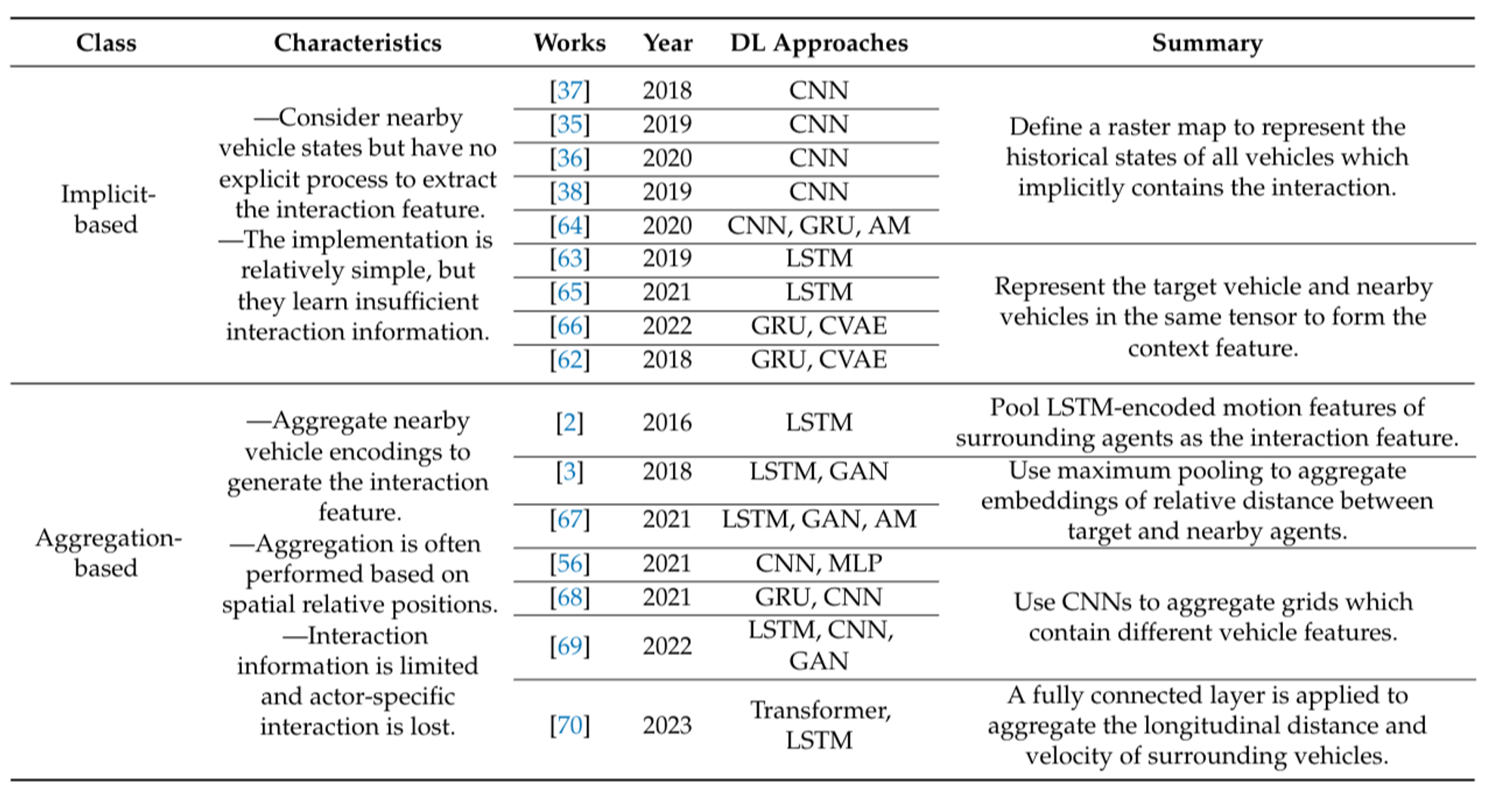
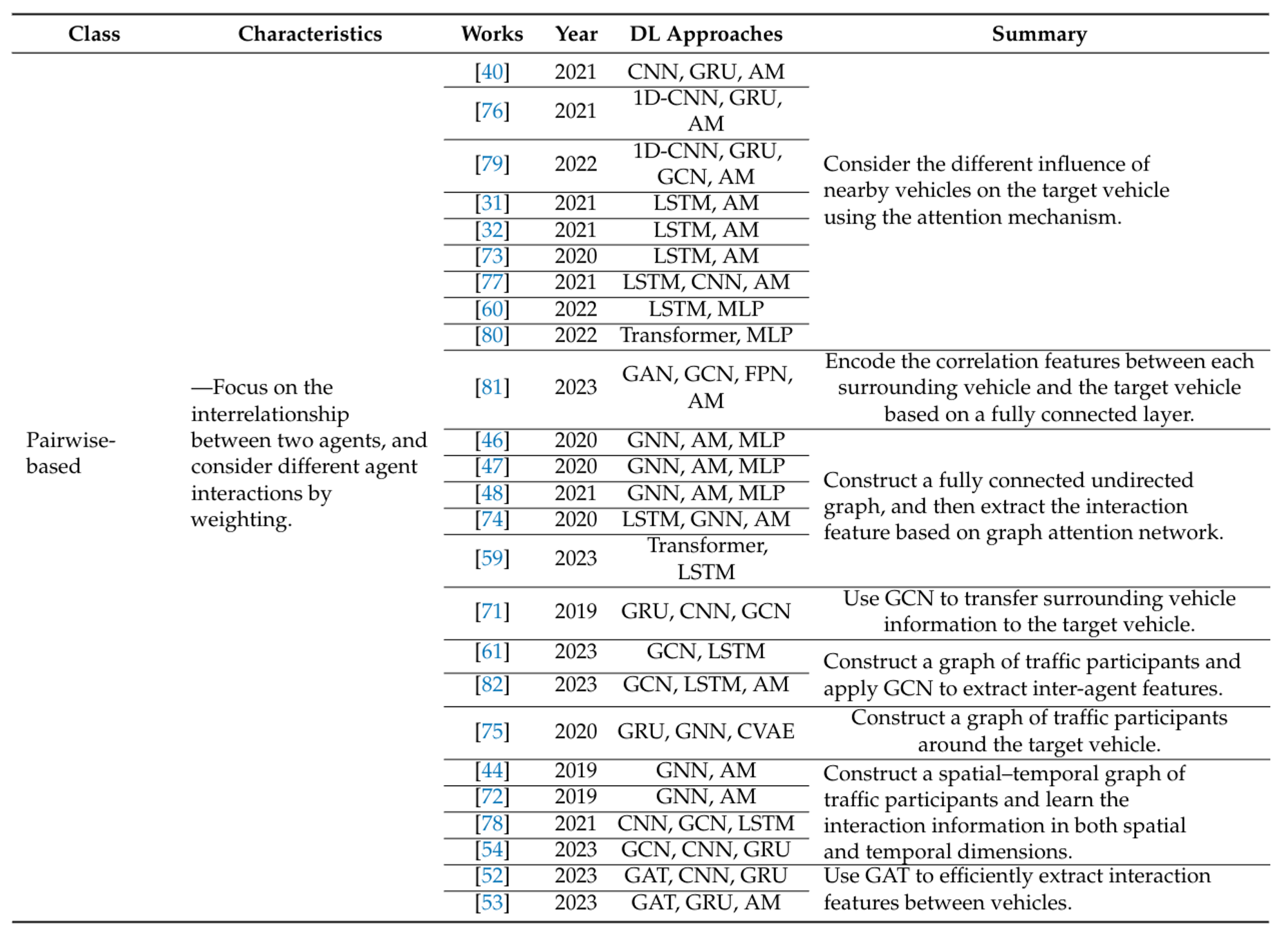Figure 10: Summary of interaction consideration methods of recent works. [1]

Map Information Fusion

Vehicle motion is constrained by map-relevant information such as road structures and traffic rules. Integrating map information into prediction models can improve prediction accuracy. Methods of map information fusion are classified into complementary fusion, coupled fusion, and guided fusion based on the mode and degree of fusion.

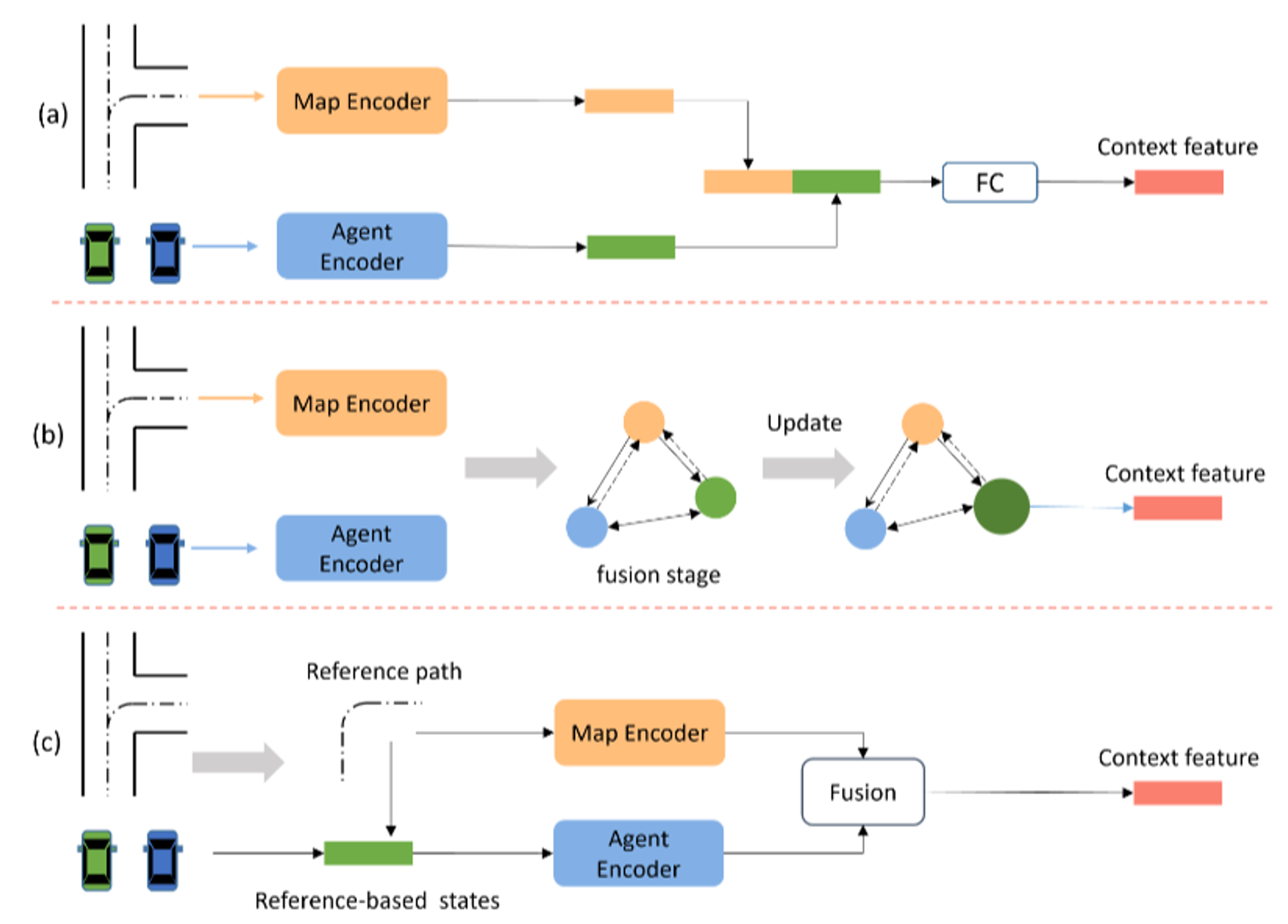Figure 11: An illustration of map information fusion methods. (a–c) represent complementary fusion, coupled fusion, and guided fusion, respectively. [1]

Complementary Fusion: This approach treats map information as an additional input supplement, encoding it independently of other motion agents. The map feature is directly concatenated with the target vehicle feature, complementing contextual information. While easy to implement and flexible in adding new map elements, this approach overlooks the connections between map elements and vehicles, limiting its ability to determine directly relevant information for the vehicle’s future motion.

Coupled Fusion: The coupled fusion approach aims for a tighter integration of map information with vehicle motion information, emphasizing the interrelationships between map elements and moving objects. Although this approach achieves adequate and efficient fusion, it complicates the addition of multiple map element types and significantly increases model complexity.

Guided Fusion: Primarily used in multimodal trajectory prediction, guided fusion considers the future lane of the target vehicle as a reference to constrain the vehicle state representation. This reference-based feature helps extract the scene context of the target vehicle while constraining the prediction region. The effectiveness of this approach heavily depends on the accuracy of the candidate lanes generated in the first stage, reflecting the vehicle’s movement intention.

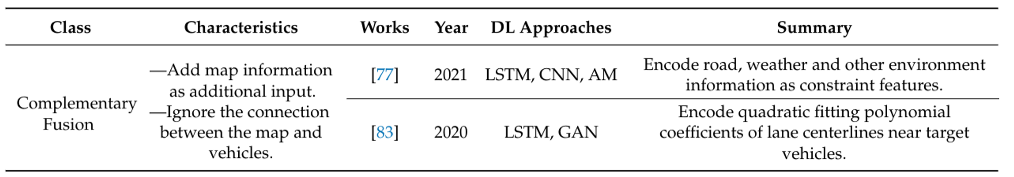
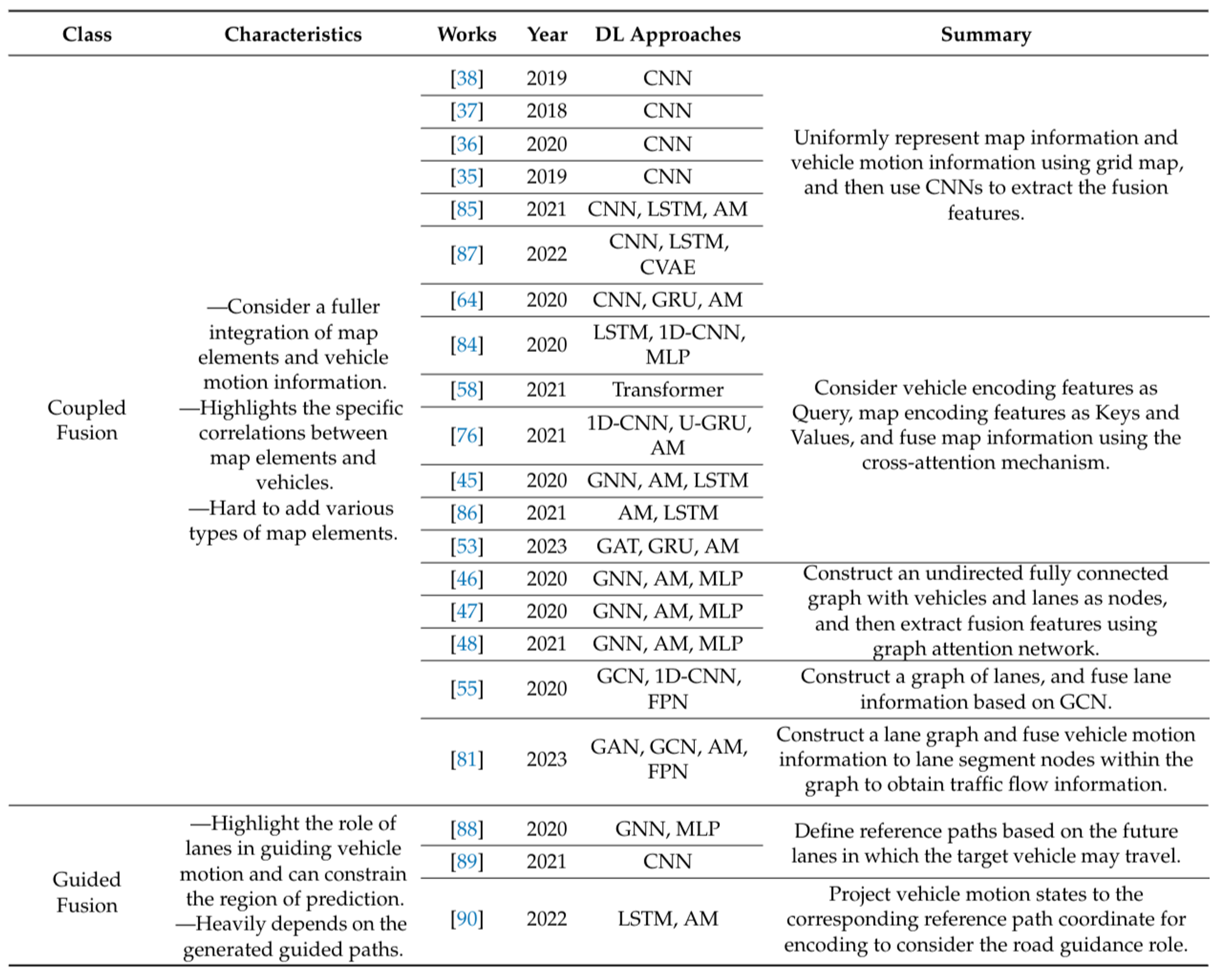Figure 12: Summary of map information fusion methods of recent works. [1]

Prediction rationality improvement

The prediction model must ensure that the prediction results of the target vehicle are not only physically safe and feasible but also semantically interpretable in real scenarios. This requirement is referred to as prediction rationality. This section summarizes the improvement methods for prediction rationality from three aspects: multimodal prediction, multi-agent joint prediction, and feasibility improvement.

Multimodal Prediction

Surrounding vehicles’ driving intentions are often unknowable, making the motion of target vehicles highly uncertain or multimodal. Vehicles with consistent historical observation states may have different future trajectories. The prediction model should explain this multimodal nature, and many works output predictions covering multiple possible motion states. However, since only one ground truth exists for model training, many multimodal learning methods are based on the winner-takes-all (WTA) approach in multi-choice learning. This section divides multimodal prediction methods into generative-based, prior-based, proposal-based, and implicit-based classes.

Generative-Based: Generative-based multimodal prediction follows a random sampling approach, primarily using Generative Adversarial Network-based (GAN-based) and Conditional Variational Auto Encoder-based (CVAE-based) methods. GAN-based methods sample noise variables to represent different modes, while CVAE-based methods generate latent variables related to the target vehicle’s historical and future motion. These methods construct low-level latent variables to obtain multiple modes through random sampling. However, they face challenges such as the uncertainty of sample diversity, poor interpretability, and the “mode collapse” problem. Additionally, predicted multimodal trajectories often lack corresponding probability values, impacting interpretability.

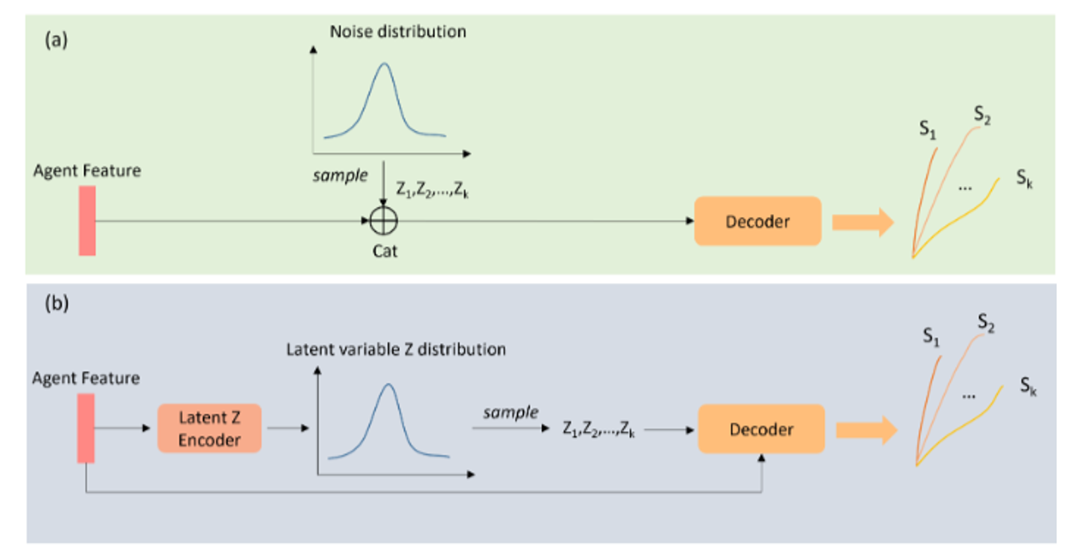Figure 13: A schematic diagram of generative-based multimodal prediction approach: (a,b) represents the process of generating multimodal trajectories in the inference stage by the GAN-based method and CVAE-based method, respectively. (a) the GAN-based method randomly samples the noise Zk with known distribution (e.g., Gaussian distribution) to represent different modes. (b) the CVAE-based method needs to encode the agent feature into a low-dimensional latent variable that obeys a predefined distribution type. Different latent variables thus are sampled based on the learned distribution and are decoded along with the agent feature to predict multimodal trajectories. [1]

Prior-Based: Prior-based multimodal prediction addresses the interpretability issue by specifying modes based on prior knowledge, such as driving maneuvers or intentions. This method predicts future motion states for each predefined mode, providing a degree of interpretability. However, it lacks the capability for multi-scene generalization and often results in a lack of diversity in multimodal outputs, as defining complete priors for future motion prediction is challenging.

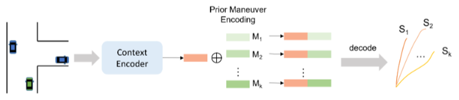Figure 14: A schematic diagram of prior-based multimodal prediction approach. The predefined prior maneuver encodings concatenate with the context feature of the target agent and then are decoded to generate trajectories of different maneuvers. [1]

Proposal-Based: The proposal-based approach generates “proposals” to guide the multimodal prediction process. These proposals can be physical quantities, such as points on lanes, or abstract quantities, such as semantic tokens. The model generates these proposals based on scene information, then predicts multimodal trajectories by decoding proposal-based features. This approach is adaptive to different scenes and can predict probabilistic values for different modes, making it widely used in recent works.

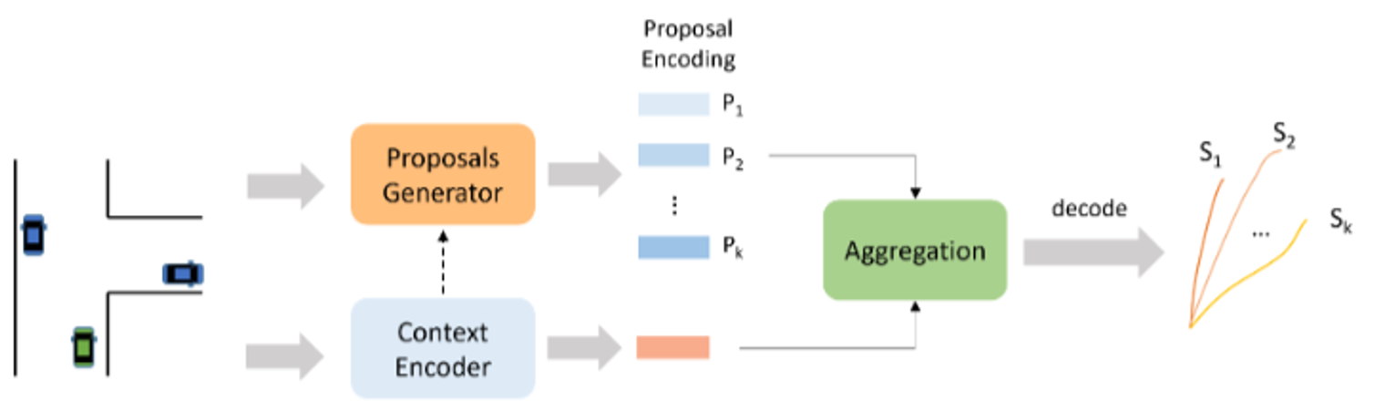Figure 15: A schematic diagram of proposal-based multimodal prediction approach. This approach requires the model to adaptively generate multiple proposals to represent different modalities based on the scenario information. [1]

Implicit-Based: The implicit-based multimodal approach assumes that the context feature extracted by the context encoder already contains multimodal information. Models of this type decode multiple possible trajectories without explicitly defining feature extraction for each mode. Although simpler to implement, this approach lacks interpretability and often provides insufficient modal diversity due to the fixed number of modalities determined before training.

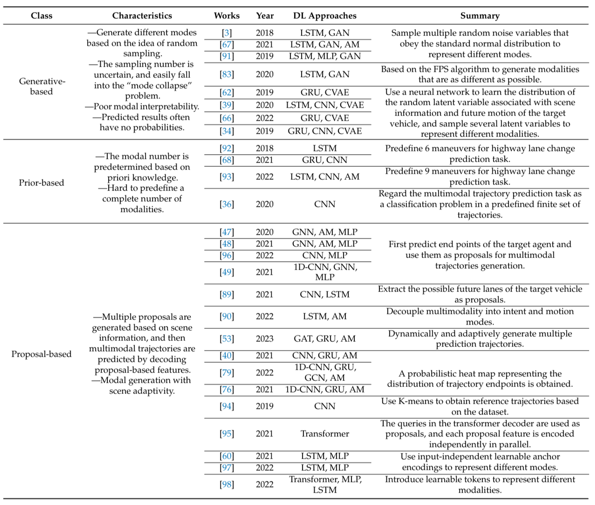
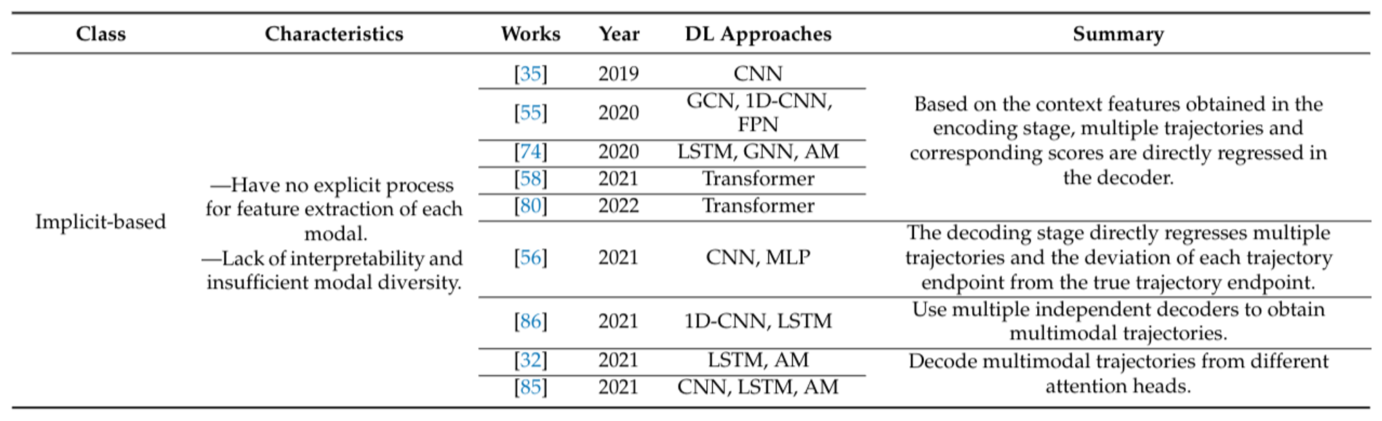Figure 16: Summary of multimodal motion prediction methods of recent works. [1]

Multi-Agent Joint Prediction

Autonomous vehicles encounter various target vehicles in real-world traffic scenarios. While many models consider multiple agents during the input stage, most predict only one target agent at a time. Joint prediction of multiple target agents is more practical. Current approaches are categorized into naive joint prediction and scene-level joint prediction.

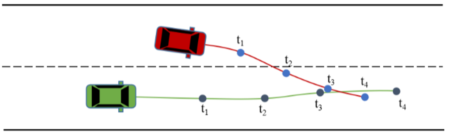Figure 17: An invalid result of naive multi-agent joint prediction. Due to the lack of consideration of coordination in the prediction stage, the green vehicle’s trajectory will overlap with the red vehicle’s trajectory at timestep t3. [1]

Naïve-Level Joint Prediction: Naïve-level joint prediction assumes that if interaction information is well-learned, the extracted context feature contains future motion information for all target agents. This approach directly regresses future motion trajectories of multiple target agents based on the scene context. It employs multi-agent loss to train the model to predict multiple agents in parallel. However, it only considers interactions from historical information and lacks coordination among agents in the prediction stage, which may lead to invalid results.

Scene-Level Joint Prediction: Scene-level joint prediction emphasizes that all target agents share the same spatial-temporal scenario in the near future and coordinates the forecasting results of each target agent. This approach considers agent interactions during the prediction stage, making it more computationally intensive than naive multi-agent prediction. Both approaches require well-detected and tracked target vehicles during the observation stage, which can be challenging in dense traffic scenarios due to occlusion.

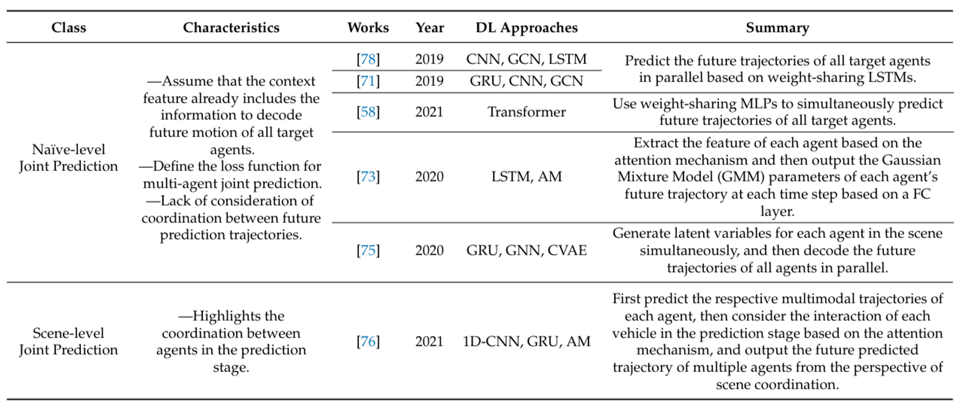Figure 18: Summary of multi-agent joint prediction methods of recent works. [1]

Feasibility Improvement

Some works treat the prediction task as a sequence translation problem, with inputs and outputs being discrete coordinate sequences of the vehicle’s center of mass. Despite the discrete nature of predicted representations, vehicle motion continuity must be maintained. Predicted trajectories should adhere to physical constraints, such as avoiding spatial overlap of multi-vehicle trajectories and remaining within road boundaries. Solutions to these issues, aimed at enhancing the feasibility and robustness of the model’s predictions, are referred to as prediction feasibility improvements.

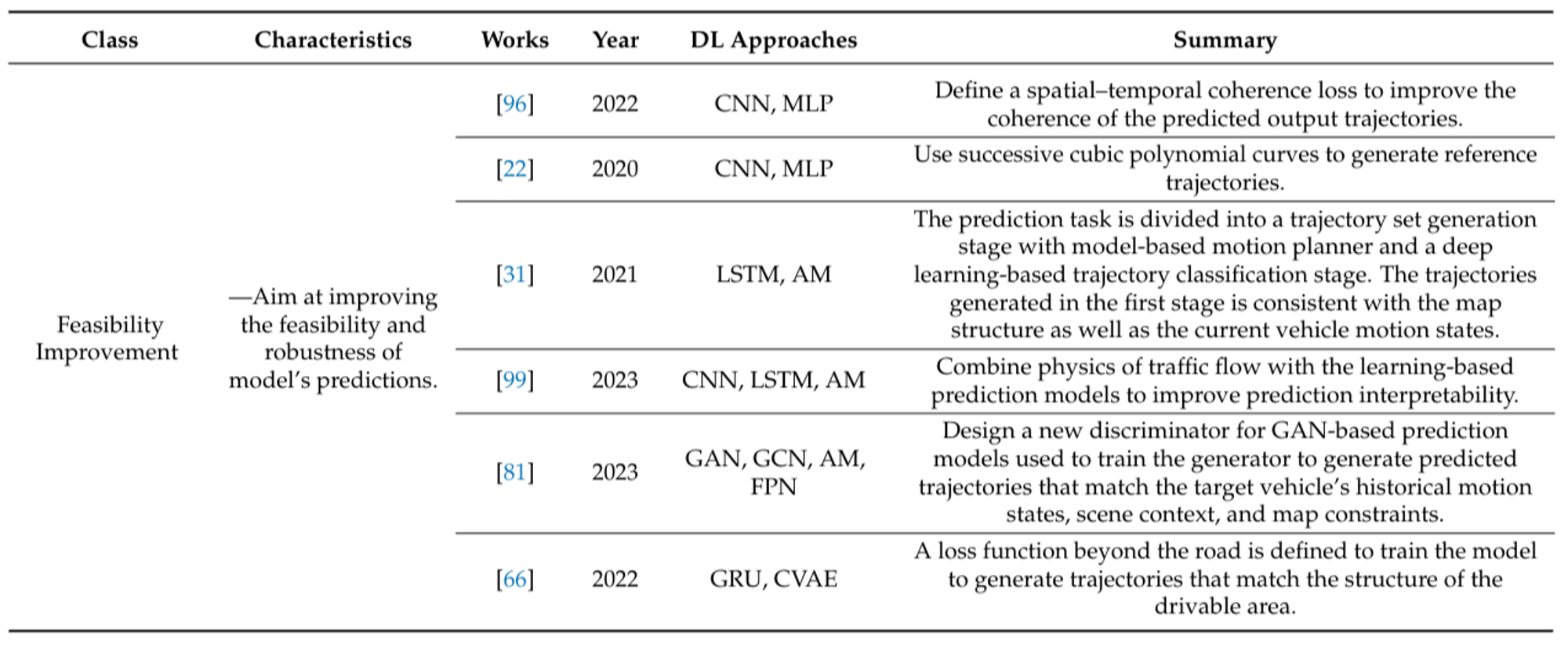Figure 19: Summary of general scene representation methods of recent works. [1]

Datasets

Datasets are critical for training and evaluating motion prediction models in autonomous driving. They provide rich, annotated data that capture various driving scenarios, enabling models to learn from real-world examples. Here are some of the main datasets used in the field:

1. NuScenes: NuScenes is a pioneering dataset that utilizes a complete suite of sensors, including six cameras, five radars, and one lidar, covering a 360-degree perception region around the vehicle. Collected in dense urban scenarios in Singapore and Boston, the NuScenes prediction dataset includes over 1000 scenes, each 20 seconds long. It provides detailed 3D coordinates, size, orientation, and map information of traffic participants, making it a comprehensive resource for motion prediction research.

2. Argoverse: Argoverse is specifically designed for tracking and trajectory prediction in autonomous driving. It offers two versions of its motion prediction dataset: Argoverse 1 and Argoverse 2. The latter is an enhanced version with richer data and more diverse scenarios. Argoverse contains various driving scenarios, such as intersections, unprotected turns, and lane changes, and provides historical tracking information along with high-definition (HD) maps. Argoverse 1, frequently used in motion prediction research, includes over 300,000 scenarios from Miami and Pittsburgh, each capturing the 2D bird’s-eye view (BEV) centroids of objects at 10 Hz. The task involves predicting future trajectories for the next 3 seconds based on 2 seconds of past observations and HD map features.

3. Waymo Open Motion Dataset (WOMD): The Waymo Open Motion Dataset is focused on dense urban driving and includes rich and challenging data records. WOMD features complex interactions and critical situations such as merging, overtaking, and unprotected turns, often involving multiple types of traffic participants simultaneously. Collected with five LiDARs and five high-resolution pinhole cameras, WOMD provides over 570 hours of data, making it one of the most extensive datasets available. It includes 1.1 million examples from urban and suburban environments, capturing diverse driving scenarios and interactions.

These datasets, along with their benchmarks, provide the foundation for developing and evaluating advanced motion prediction models, helping researchers address the complexities and dynamics of real-world driving environments.

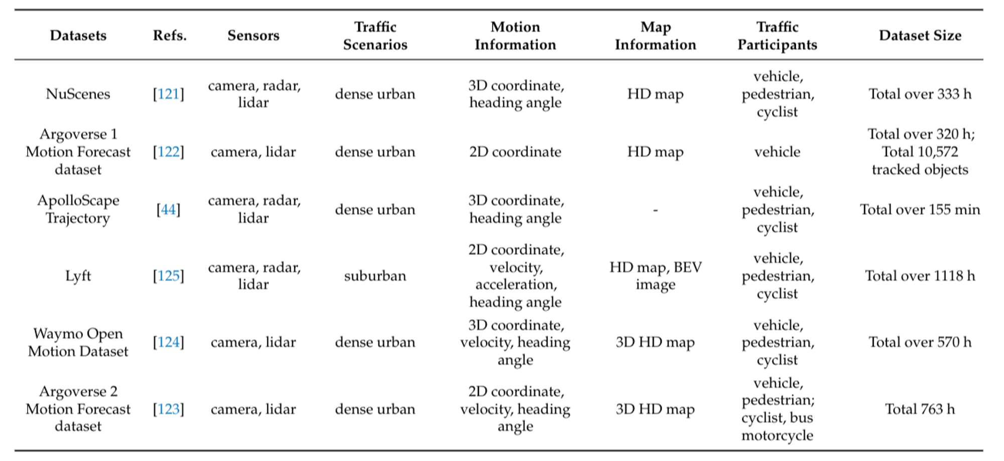Figure 20: Motion prediction datasets. [1]

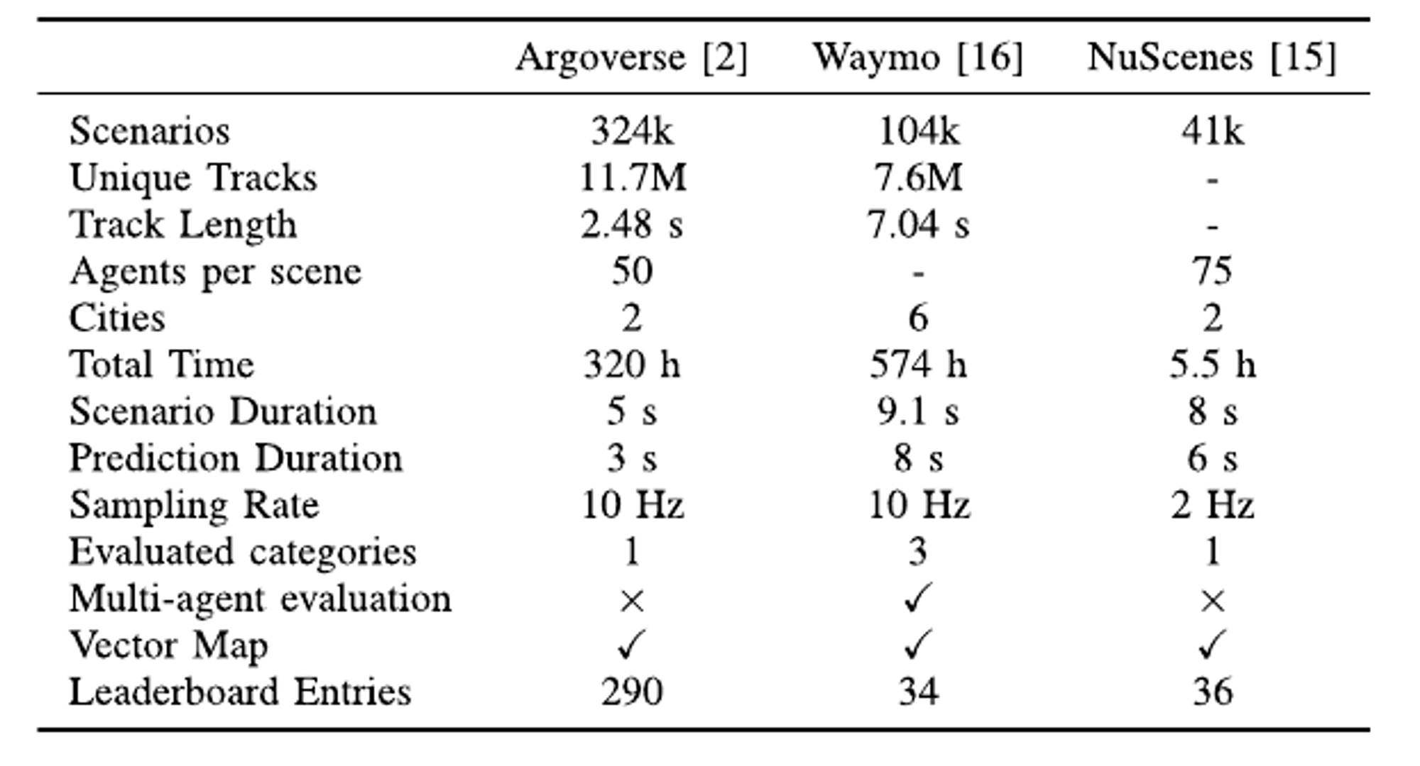Figure 21: Comparison between popular benchmark for vehicle motion prediction. Track length and agents per scene represent average values per scenario. Learderboard entries values retrivied on January 13, 2023. [3]

Evaluation metrics

Evaluation metrics play a crucial role in assessing the performance of motion prediction models in autonomous driving. Here, we focus on trajectory-based metrics, categorized into displacement metrics for single-modal, multimodal, and multi-agent joint predictions, as well as other metrics for trajectory prediction.

Displacement Metrics for Single-Modal Prediction

1. Final Displacement Error (FDE): FDE calculates the L2 distance between the predicted trajectory’s endpoint and the ground truth endpoint. This metric evaluates the accuracy of the endpoint prediction, which is critical as it relates to the vehicle’s intended final position.

\[\begin{equation} \text{FDE} = \sqrt{(x_{T_{\text{pred}}} - x_{T_{\text{pred}}}^{\text{gt}})^2 + (y_{T_{\text{pred}}} - y_{T_{\text{pred}}}^{\text{gt}})^2} \end{equation}\]

2. Average Displacement Error (ADE): ADE measures the overall distance deviation of the predicted trajectory from the ground truth trajectory over the prediction horizon.

\[\begin{equation} \text{ADE} = \frac{1}{T_{\text{pred}}} \sum_{t=1}^{T_{\text{pred}}} \sqrt{(x_t - x_t^{\text{gt}})^2 + (y_t - y_t^{\text{gt}})^2} \end{equation}\]

3. Root Mean Square Error (RMSE): RMSE calculates the average of the squared distances between the predicted and ground truth trajectories, providing a measure of the prediction accuracy over the entire trajectory.

\[\begin{equation} \text{RMSE} = \sqrt{\frac{1}{T_{\text{pred}}} \sum_{t=1}^{T_{\text{pred}}} [(x_t - x_t^{\text{gt}})^2 + (y_t - y_t^{\text{gt}})^2]} \end{equation}\]

4. Mean Absolute Error (MAE): MAE is the average of the absolute errors between the predicted and ground truth trajectories. It is computed separately for the horizontal (x) and vertical (y) directions.

\[\begin{equation} \text{MAE}_x = \frac{1}{T_{\text{pred}}} \sum_{t=1}^{T_{\text{pred}}} |x_t - x_t^{\text{gt}}| \end{equation}\] \[\begin{equation} \text{MAE}_y = \frac{1}{T_{\text{pred}}} \sum_{t=1}^{T_{\text{pred}}} |y_t - y_t^{\text{gt}}| \end{equation}\]

Displacement Metrics for Multimodal Prediction

1. Minimum Final Displacement Error (\(minFDE_K\)): \(minFDE_K\) represents the minimum FDE among \(K\) predicted trajectories. This metric ensures that at least one of the predicted trajectories is close to the ground truth.

2. Minimum Average Displacement Error (\(minADE_K\)): \(minADE_K\) is the minimum ADE among \(K\) predicted trajectories. In Argoverse, \(minADE_K\) corresponds to the ADE of the trajectory with the minimum FDE, ensuring consistency of the optimal predicted trajectory.

3. Brier Score-Based Metrics:

• \(brier\_minFDE_K\): Adds \((1 - p)^2\) to \(minFDE_K\), where \(p\) is the predicted probability of the optimal trajectory.
• \(brier\_minADE_K\): Adds \((1 - p)^2\) to \(minADE_K\), emphasizing the probability confidence of the optimal trajectory.

Displacement Metrics for Multi-Agent Joint Prediction

When predicting multiple target agents, the corresponding metrics are extensions of single-agent metrics, considering the average values across multiple agents.

1. \(ADE(N_{TV})\): Average ADE for \(N_{TV}\) target vehicles.

2. \(FDE(N_{TV})\): Average FDE for \(N_{TV}\) target vehicles.

3. \(min\_ADE(N_{TV})\): Minimum ADE for \(N_{TV}\) target vehicles.

4. \(min\_FDE(N_{TV})\): Minimum FDE for \(N_{TV}\) target vehicles.

Other Metrics for Trajectory Prediction

Beyond displacement metrics, other metrics are used to evaluate different aspects of trajectory prediction:

1. Miss Rate (MR): MR measures the ratio of predicted trajectories whose endpoints deviate from the true endpoint by more than a specified threshold (d). MR reflects the model’s overall accuracy in predicting the trajectory endpoint.

2. Overlap Rate (OR): OR assesses the physical feasibility of the prediction model. If the predicted trajectory of an agent overlaps with another agent’s trajectory at any timestep, it is considered an overlap. OR is the ratio of overlapped trajectories to all predicted trajectories.

3. Mean Average Precision (mAP): mAP, introduced in the Waymo Open Motion Dataset, evaluates the accuracy and recall of multimodal trajectory predictions. It groups target agents by the shape of their future trajectories and calculates the average precision within each group. The final mAP is the average over all groups.

These metrics provide a comprehensive evaluation framework for motion prediction models, addressing different prediction aspects and ensuring robust performance assessment.

Experiments

What’s next?

References

[1] Huang, R., Zhuo, G., Xiong, L., Lu, S., & Tian, W. (2023). A Review of Deep Learning-Based Vehicle Motion Prediction for Autonomous Driving. Sustainability, 15(20), 14716. https://doi.org/10.3390/su152014716

[2] Motion Forecasting (Waabi CVPR 23 Tutorial on Self-Driving Cars) - YouTube - https://www.youtube.com/watch?v=8Mr7k8fJGqE

[3] Gomez-Huelamo, C., Conde, M. v., Barea, R., Ocana, M., & Bergasa, L. M. (2023). Efficient Baselines for Motion Prediction in Autonomous Driving. IEEE Transactions on Intelligent Transportation Systems. https://doi.org/10.1109/TITS.2023.3331143

[4] Mozaffari, S., Al-Jarrah, O. Y., Dianati, M., Jennings, P., & Mouzakitis, A. (2022). Deep Learning-Based Vehicle Behavior Prediction for Autonomous Driving Applications: A Review. In IEEE Transactions on Intelligent Transportation Systems (Vol. 23, Issue 1, pp. 33–47). Institute of Electrical and Electronics Engineers Inc. https://doi.org/10.1109/TITS.2020.3012034

[5] Gulzar, M., Muhammad, Y., & Muhammad, N. (2021). A Survey on Motion Prediction of Pedestrians and Vehicles for Autonomous Driving. In IEEE Access (Vol. 9, pp. 137957–137969). Institute of Electrical and Electronics Engineers Inc. https://doi.org/10.1109/ACCESS.2021.3118224